Principal Component Analysis of the Term Structure of European Interest Rate Yields
An analysis and literature review of factor investing in fixed income, where the first three components can be attributed to actual meanings in a Bonds Portfolio setting
Overview
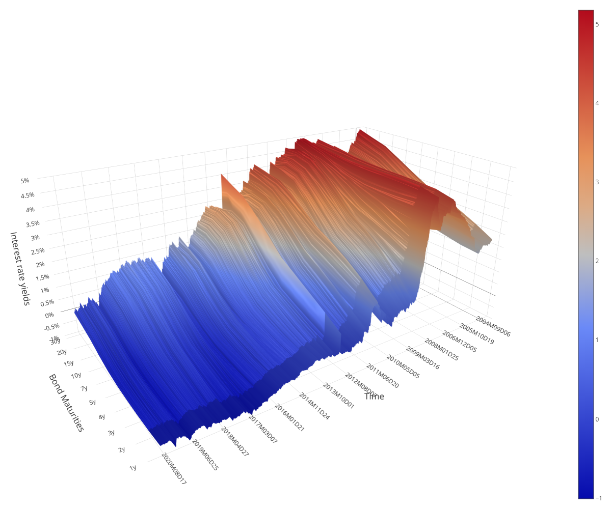
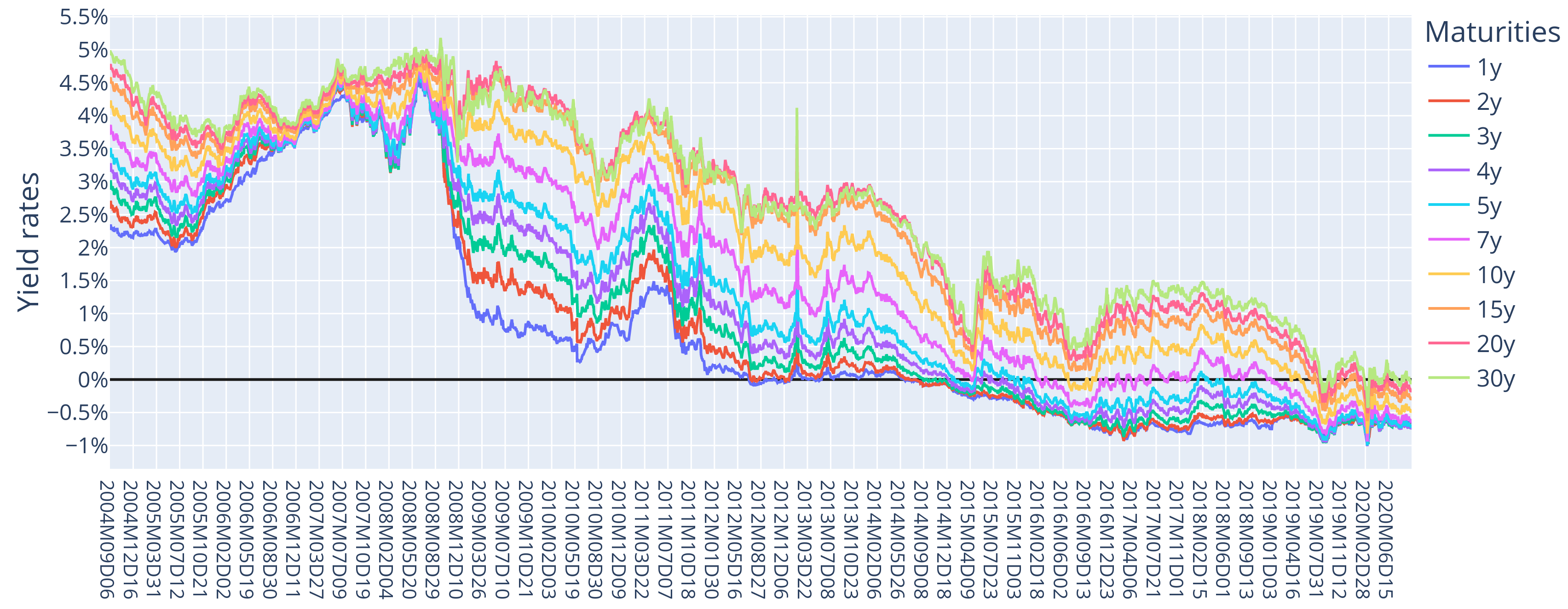
This project explores the application of Principal Component Analysis (PCA) to the term structure of European interest rate yields over the period from 2004 to 2020. The dataset includes daily interest rate yields of AAA-rated bonds from various maturities, spanning from one year to thirty years. The primary aim is to investigate the efficacy of PCA in identifying the main factors that drive changes in the yield curve, especially in different interest rate environments.
Quick PCA Math Overview
Principal Component Analysis (PCA) is a statistical technique used to simplify the complexity in high-dimensional data while retaining trends and patterns. It does this by transforming the data into a new set of variables, the principal components (PCs), which are uncorrelated and ordered so that the first few retain most of the variation present in the original dataset.
In mathematical terms, the kth principal component (PC) is given by:
\[z_k = \alpha_0^k x = \alpha_0^{k1} x_1 + \alpha_0^{k2} x_2 + ... + \alpha_0^{kp} x_p = \sum_{j=1}^p \alpha_0^{kj} x_j\]
The first PC maximizes its variance under the constraint that the sum of squared values in the first eigenvector is 1. The second PC maximizes its variance under the constraint that the sum of squared values in the second eigenvector is 1 and that the covariance between the first PC and the second PC is 0.
The first principal component (PC) is the linear combination with maximal variance:
\[\text{max : var}(z_1) = \text{var}(\alpha_0^1 x) \quad \text{s.t.} \quad \alpha_0^1 \alpha_1 = 1\]
This maximization is equivalent to:
\[\text{max :} \quad \alpha_0^1 \Sigma \alpha_1 \quad \text{s.t.} \quad \alpha_0^1 \alpha_1 = 1\]
From this, it follows a Lagrange optimization problem:
\[L = \alpha_0^1 \Sigma \alpha_1 - \lambda (\alpha_0^1 \alpha_1 - 1)\]
The solution to this optimization gives us the principal components as the eigenvectors of the covariance matrix \( \Sigma \).
Key Objectives
- PCA Application: Apply PCA to the term structure of interest rate yields to identify the primary components that explain the variability in the yield curve.
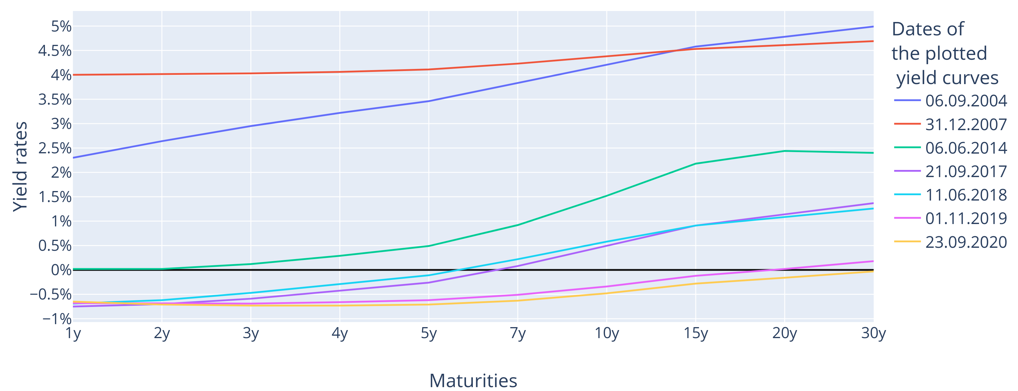
- Shift, Slope, and Curvature: Interpret the first three principal components (PCs) as shift (or level), slope (or steepness), and curvature of the yield curve, respectively.
- Interest Rate Environment Analysis: Compare the efficacy of PCA in positive and negative interest rate environments, evaluating whether the amount of variability explained by the first three PCs differs between these environments.
Methodology
- Data Collection: The dataset comprises daily yield data for AAA-rated bonds in the Euro Area, sourced from the Eurostat Database. The time series spans from September 6, 2004, to September 23, 2020.
- Data Partitioning: The data is divided into five parts for detailed analysis:
- Part 1: Entire dataset (2004-2020)
- Part 2: Positive interest rate environment (2004-2007)
- Part 3: Negative interest rate environment (2014-2017)
- Part 4: Deep negative interest rate environment (2017-2020)
- Part 5: Extended negative interest rate period (2014-2020)
- Stationarity: Ensuring stationarity of the data by taking the first differences of the yields.
- PCA Implementation: Conduct PCA on the correlation matrix of the first differences of the yield data to identify the principal components.
Findings
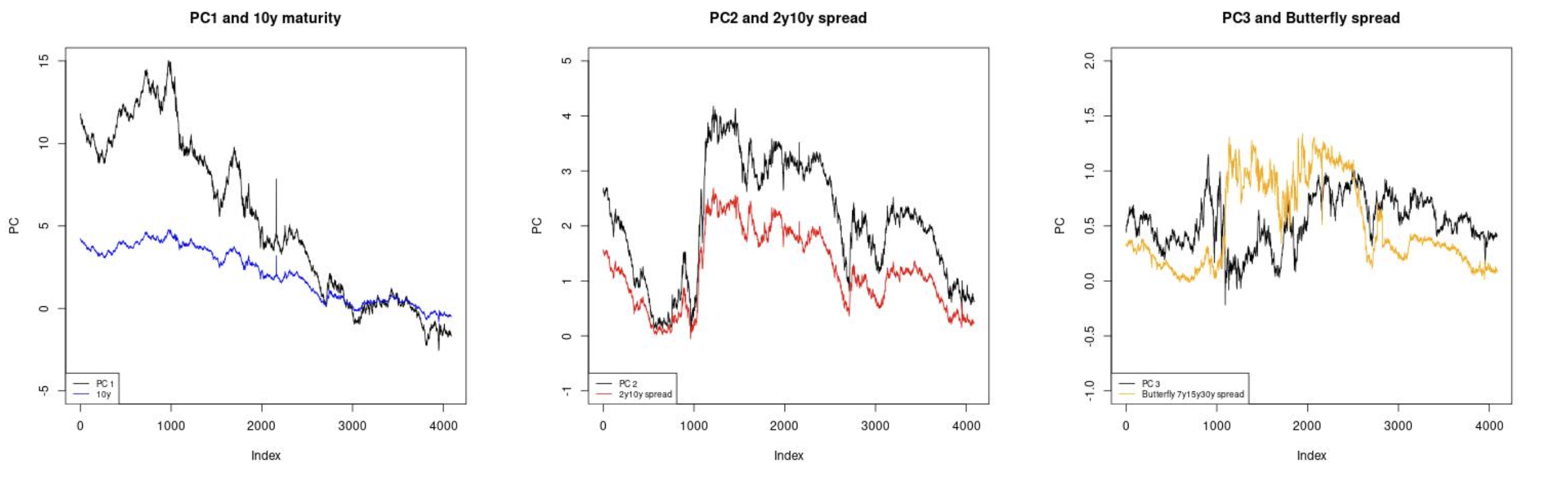
- Shift, Slope, and Curvature: The first three PCs effectively represent the shift, slope, and curvature of the yield curve, consistent with findings in previous literature.
- Interest Rate Environment: Contrary to some recent studies, this analysis finds no significant difference in the efficacy of PCA between positive and negative interest rate environments. The amount of variability explained by the first three PCs remains substantial in both cases.
Principal Components Interpretation
First Principal Component - Level/Shift
The first PC captures parallel shifts in the yield curve, representing the overall level of interest rates. This component typically explains the largest portion of yield curve variation and is closely related to monetary policy changes and general economic conditions.
Second Principal Component - Slope
The second PC represents changes in the slope of the yield curve, capturing the spread between long-term and short-term rates. This component is often associated with expectations about future economic growth and inflation.
Third Principal Component - Curvature
The third PC captures changes in the curvature of the yield curve, representing how the middle portion of the curve moves relative to the short and long ends. This is often related to specific market segments or technical factors in bond markets.
Conclusion
This project demonstrates the robustness of PCA in analyzing the term structure of interest rates. The findings suggest that PCA can reliably capture the main factors driving yield curve changes across different interest rate environments. These insights are valuable for risk management and portfolio optimization in the bond market.